Easy Deployment of Machine Learning Models with Serialization Model Classes

Training a great model can take a lot of work. Getting that model into production should be quick and easy. ADS has a set of classes that take your model and push it to production with a few quick steps.

The first step is to create a model serialization object. This object wraps your model and has a number of methods to assist in deploying it. There are different model classes for different model classes. For example, if you have a PyTorch model you would use the PyTorchModel class. If you have a TensorFlow model you would use the TensorFlowModel class. ADS has model serialization for many different model classes. However, it is not feasible to have a model serialization class for all model types. Therefore, the GenericModel can be used for any class that has a .predict() method.

Read More: Database Certifications

After creating the model serialization object, the next step is to use the .prepare() method to create the model artifacts. The score.py file is created and it is customized to your model class. You may still need to modify it for your specific use case but this is generally not required. The .prepare() method also can be used to store metadata about the model, code used to create the model, input and output schema, and much more.

If you make changes to the score.py file, call the .verify() method to confirm that the load_model() and predict() functions in this file are working. This speeds up your debugging as you do not need to deploy a model to test it.

The .save() method is then used to store the model in the model catalog. A call to the .deploy() method creates a load balancer and the instances needed to have an HTTPS access point to perform inference on the model. Using the .predict() method, you can send data to the model deployment endpoint and it will return the predictions.

This blog post uses a TensorFlow model as its example. The process for the other serialization model classes is the same.

The TensorFlowModel class in ADS is designed to allow you to rapidly get a TensorFlow model into production. The .prepare() method creates the model artifacts that are needed to deploy a functioning model without you having to configure it or write code. However, you can customize the required score.py file.

The following steps take your trained TensorFlow model and deploy it into production with a few lines of code.

Create a Model

The first step is to create a model that you wish to deploy.

Initialize

Instantiate a TensorFlowModel() object with a TensorFlow model. Each instance accepts the following parameters:

◉ artifact_dir: str: Artifact directory to store the files needed for deployment.

◉ auth: (Dict, optional): Defaults to None. The default authentication is set using the ads.set_auth API. To override the default, use ads.common.auth.api_keys() or ads.common.auth.resource_principal() and create the appropriate authentication signer and the **kwargs required to instantiate the IdentityClient object.

◉ estimator: Callable: Any model object generated by the TensorFlow framework.

◉ properties: (ModelProperties, optional): Defaults to None. The model properties that are used to save and deploy the model.

By default, properties is populated from the appropriate environment variables if it’s not specified. For example, in a notebook session, the environment variables for project id and compartment id are preset and stored in PROJECT_OCID and NB_SESSION_COMPARTMENT_OCID by default. So properties populates these variables from the environment variables and uses the values in methods such as .save() and .deploy(). However, you can explicitly pass in values to overwrite the defaults. When you use a method that includes an instance of properties, then properties records the values that you pass in. For example, when you pass inference_conda_env into the .prepare() method, then properties records this value. To reuse the properties file in different places, you can export the properties file using the .to_yaml() method and reload it into a different machine using the .from_yaml() method.

Summary Status

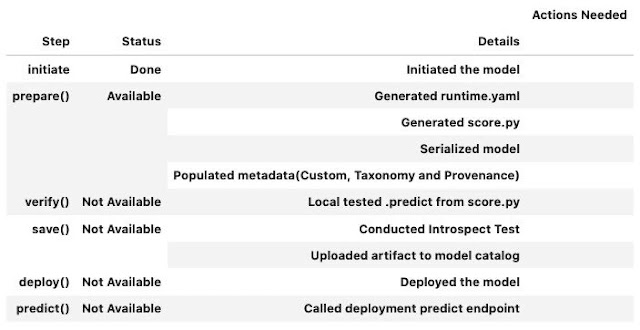
You can call the .summary_status() method after a model serialization instance such as AutoMLModel, GenericModel, SklearnModel, TensorFlowModel, or PyTorchModel is created. The .summary_status() method returns a Pandas dataframe that guides you through the entire workflow. It shows which methods are available to call and which ones aren’t. Plus it outlines what each method does. If extra actions are required, it also shows those actions.

The following image displays an example summary status table created after a user initiates a model instance. The table’s Step column displays a Status of Done for the initiate step. And the Details column explains what the initiate step did such as generating a score.py file. The Step column also displays the prepare(), verify(), save(), deploy(), and predict() methods for the model. The Status column displays which method is available next. After the initiate step, the prepare() method is available. The next step is to call the prepare() method.

Model Deployment

Prepare

The prepare step is performed by the .prepare() method. It creates several customized files used to run the model after it is deployed. These files include:

◉ input_schema.json: A JSON file that defines the nature of the features of the X_sample data. It includes metadata such as the data type, name, constraints, summary statistics, feature type, and more.

◉ model.h5: This is the default filename of the serialized model for PyTorch models. Other serialization models use different formats and the file extension is changed to reflect this. You can change it with the model_file_name attribute. You can use the as_onnx parameter to save it in the ONNX format.

◉ output_schema.json: A JSON file that defines the nature of the dependent variable in the y_sample data. It includes metadata such as the data type, name, constraints, summary statistics, feature type, and more.

◉ runtime.yaml: This file contains information that is needed to set up the runtime environment on the deployment server. It has information about which conda environment was used to train the model, and what environment should be used to deploy the model. The file also specifies what version of Python should be used.

◉ score.py: This script contains the load_model() and predict() functions. The load_model() function understands the format the model file was saved in, and loads it into memory. The .predict() method is used to make inferences in a deployed model. There are also hooks that allow you to perform operations before and after inference. You are able to modify this script to fit your specific needs.

The .prepare() method serializes the model and prepares and saves the score.py and runtime.yaml files.

Verify

If you update the score.py file included in a model artifact, you can verify your changes, without deploying the model. With the .verify() method, you can debug your code without having to save the model to the model catalog and then deploying it. The .verify() method takes a set of test parameters and performs the prediction by calling the predict() function in score.py. It also runs the load_model() function to load the model.

The verify() method tests whether the .predict() API works in the local environment.

In TensorFlowModel, data serialization is supported for JSON serializable objects. Plus, there is support for a dictionary, string, list, np.ndarray, and tf.python.framework.ops.EagerTensor. Not all these objects are JSON serializable, however, support to automatically serializes and deserialized is provided. What data formats depend on the serialization model class. However, the generally support objects that are JSON serializable. Check the documentation for what formats are support for each serialization model class.

Save

After you are satisfied with the performance of your model and have verified that the score.py file is working, use the .save() method to save the model to the model catalog. The .save() method bundles up the model artifacts, stores them in the model catalog, and returns the model OCID.

The .save() method stores the model artifacts in the model catalog.

The .save() method reloads score.py and runtime.yaml files from disk. This will pick up any changes that have been made to those files. If ignore_introspection=False then it conducts an introspection test to determine if the model deployment might have issues. If potential problems are detected, it will suggest possible remedies. Lastly, it uploads the artifacts to the model catalog, and returns the model OCID. You can also call .instrospect() to conduct the test any time after you call .prepare().

Deploy

You can use the .deploy() method to deploy a model. You must first save the model to the model catalog, and then deploy it.

The .deploy() method returns a ModelDeployment object. Specify deployment attributes such as display name, instance type, number of instances, maximum router bandwidth, and logging groups.

Predict

To get a prediction for your model, after your model deployment is active, call the .predict() method. The .predict() method sends a request to the deployed endpoint, and computes the inference values based on the data that you input in the .predict() method.

The .predict() method returns a prediction of input data that is run against the model deployment endpoint.

Delete a Deployment

Use the .delete_deployment() method on the serialization model object to delete a model deployment. You must delete a model deployment before deleting its associated model from the model catalog.

Each time you call the .deploy() method, it creates a new deployment. Only the most recent deployment is attached to the object.

The .delete_deployment() method deletes the most recent deployment.

Example

import tempfile

import tensorflow as tf

from ads.catalog.model import ModelCatalog

from ads.common.model_metadata import UseCaseType

from ads.model.framework.tensorflow_model import TensorFlowModel

mnist = tf.keras.datasets.mnist

(x_train, y_train), (x_test, y_test) = mnist.load_data()

x_train, x_test = x_train / 255.0, x_test / 255.0

model = tf.keras.models.Sequential(

    [

        tf.keras.layers.Flatten(input_shape=(28, 28)),

        tf.keras.layers.Dense(128, activation="relu"),

        tf.keras.layers.Dropout(0.2),

        tf.keras.layers.Dense(10),

])

loss_fn = tf.keras.losses.SparseCategoricalCrossentropy(from_logits=True)

model.compile(optimizer="adam", loss=loss_fn, metrics=["accuracy"])

model.fit(x_train, y_train, epochs=1)

# Deploy the model, test it and clean up.

artifact_dir = tempfile.mkdtemp()

tensorflow_model = TensorFlowModel(estimator=model, artifact_dir= artifact_dir)

tensorflow_model.prepare(

    inference_conda_env="generalml_p37_cpu_v1",

    training_conda_env="generalml_p37_cpu_v1",

    use_case_type=UseCaseType.MULTINOMIAL_CLASSIFICATION,

    X_sample=x_test,

    y_sample=y_test,

)

tensorflow_model.verify(x_test[:1])

model_id = tensorflow_model.save()

tensorflow_model_deployment = model.deploy()

tensorflow_model.predict(x_test[:1])

tensorflow_model.delete_deployment(wait_for_completion=True)

ModelCatalog(compartment_id=os.environ['NB_SESSION_COMPARTMENT_OCID']).delete_model(model_id)

Source: oracle.com